Statistiek Kennisonderwerp

• Een test met een hoge sensitiviteit kan goed gebruikt worden om ziekten uit te sluiten bij een negatieve uitslag.
  • fractie terecht positieven onder alle zieke personen
• Een test met een hoge specificiteit kan goed gebruikt worden om ziekten aan te tonen bij een positieve uitslag. 
  • terecht negatieven onder niet-zieke personen
  • 100% specifieke test: 0% fout-positieven, dus positieve testuitslag geeft zekerheid over ziekte.
• Bij toenemende prevalentie zal de positief-voorspellende waarde van de test toenemen. Aangezien sensitiviteit en specificiteit afhankelijk van de test zijn en niet van de populatie, veranderen deze niet bij wisselende prevalenie.
• Sens/spec meer in onderzoekssetting (in screeningssetting) -> hoe ga je niet teveel mensen missen?
  • Kun je ook zien als: veiligheid en efficiëntie
• Infographic uitleg HenW link

Sensitiviteit

is de gevoeligheid van een test in de medische diagnostiek, dat wil zeggen hoe goed de test erin slaagt datgene aan te tonen wat van de test verwacht wordt.
= terecht positieve uitslagen onder de zieke personen/totaal aantal zieke personen. Risico: veel vals-positieven.
De kans dat een persoon die de aandoening heeft, een positieve testuitslag heeft

Specificiteit

bepaalt hoe specifiek de test is, dat wil zeggen hoe goed de test erin slaagt de afwezigheid van het verschijnsel aan te tonen.
= terecht negatieve uitslagen onder niet-zieke personen/totaal aantal niet-zieke personen.
De kans dat een persoon die de aandoening niet heeft, een negatieve testuitslag heeft

Positieve voorspellende

waarde wordt gewenst hoog te zijn als een medische behandeling schadelijk zou kunnen zijn. Er worden dan wel een aantal patiënten gemist die een fout-negatieve uitslag hebben. Deze mensen moeten dan met een andere test worden opgespoord.
De kans dat iemand met een positieve test de ziekte echt heeft

Negatief voorspellende waarde

Als een ziekte beslist niet gemist mag worden, dan is een test met een hoge negatief voorspellende waarde gewenst. Hierdoor worden er ook een aantal patiënten behandeld die een fout-positieve testuitslag hebben, maar de behandeling is in een dergelijk geval niet schadelijk voor de patiënt.
De kans dat iemand met een negatieve test de ziekte echt niet heeft

test positief	A (Echt-positieven, TP)	B (Fout-positieven, FP)	TP+FP	PVW = TP/(TP+FP)
test negatief	C (Fout-negatieven, FN)	D (Echt-negatieven, TN)	TN+FN	NVW = TN/(TN+FN)
totaal	TP+FN	FP+TN
formule	Sens = TP/(TP+FN)	Spec = TN/(FP+TN)

Number needed to treat (NNT)

Het NNT is de inverse van de absolute risicoreductie ARR

Alle termen

• Absolute risicoreductie (ARR): Risicoverschil. Verschil in absolute risico op de uitkomst tussen de interventiegroep en controlegroep. ARR = AR controle – AR interventie
• Relatieve risico (RR): Verhouding van het absolute risico op de uitkomst tussen interventiegroep en controlegroep. RR = AR interventie / AR controle
• Relatieve risicoreductie (RRR): Verhouding van het risicoverschil tussen de interventiegroep en de controlegroep ten opzichte van het risico in de controlegroep
• RRR = (AR controle – AR interventie) / AR controle
• Number needed to treat (NNT): Aantal patiënten dat met de interventie behandeld dient te worden om 1 gewenste gebeurtenis meer te bereiken dan met de controlebehandeling verkregen zou zijn. NNT = 1/ARR
• Number needed to harm (NNH): Aantal patiënten dat met de interventie behandeld dient te worden om 1 ongewenste gebeurtenis (bijwerking) meer te bereiken dan met de controlebehandeling verkregen zou zijn. NNH = 1/ARR
• Prevalentie vs Incidentie
  • Prevalentie: bestaande gevallen, incidentie: nieuwe gevallen

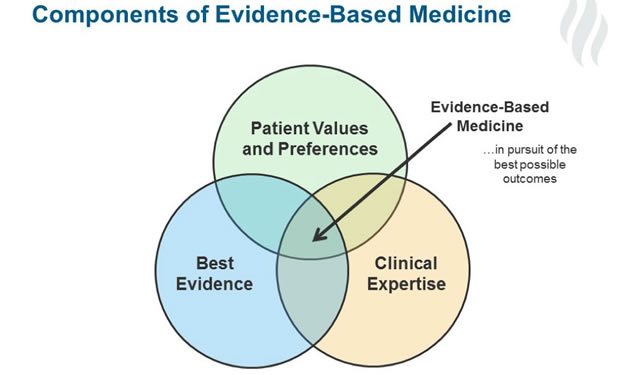
Evidence based medicine

Systematic review

Funnel plot

• https://www.bmj.com/content/343/bmj.d4002
• A funnel plot for this analysis (Figure 5) was reasonably symmetrical, suggesting the absence of important bias or small-study effects in the set of studies.
  

Comprehensive cohort design (CCD) / patient preference trial^[1]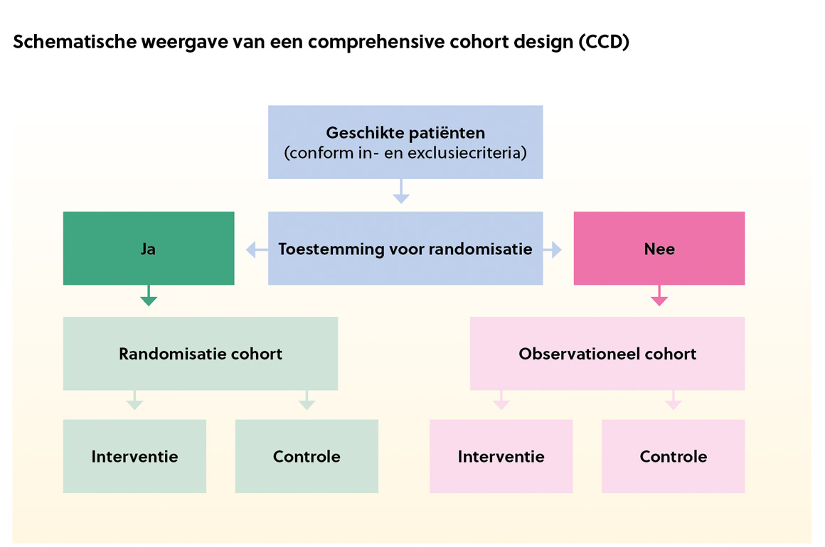

Hybride: RCT gecombineerd met prospectief onderzoek

• opgebouwd uit twee cohorten
  • één randomisatiecohort, waarin patiënten zonder dominante behandelvoorkeur worden geïncludeerd
  • één observationeel prospectief cohort, waarin geschikte patiënten maar met een behandelvoorkeur worden opgenomen

Statistische tests en uitvoering in SPSS

Independent t-test →Comparing the means of 2 conditions with different test-subjects.

• Analyze → compare means → independent-sample t test.

Dependent t-test → Comparing the means of 2 conditions with the same entities (test-subjects).

• Analyze → compare means → paired-samples t test

One-way ANOVA → Comparing 2 or more independent means.

• Analyze → general linear model → univariate OR Analyze → compare means → one-way ANOVA
• Options → descriptive statistics and homogeneity tests

Factorial ANOVA → Comparing multiple means when there are 2 or more independent variables.

• Analyze → general linear model → univariate → place the independent variable(s) in fixed factor(s)
• Options → descriptive statistics and homogeneity tests

ANCOVA →Exclude the influence of covariates on the dependent variable.

• Analyze → general linear model → univariate → place DV in dependent variable, IV in fixed factor(s) and covariate in covariate(s).
• EM means → move the IV to display means for.

This will show the means adjusted for the covariate (they will be closer together). Mixed ANOVA →Comparing multiple means when there are 2 or more independent variables (time of measurement and intervention) that use both a within-subject factor (time of measurement) and between-subjects factor (intervention).

• Analyze → general linear model → repeated measures.
• Define the within-subjects IV (time of measurement) by giving it a name in within-subject factor name → fill in the number of groups it contains in number of levels → add → define.
• Drag the ‘group’ IV to between-subjects factor(s) and the ‘measurement moment’ IVs to within- subjects variables.
• Plots →drag the ‘measurement moment’ IV to horizontal axis and the ‘group’ IV to separate lines.

Simple linear regression analysis →Testing if x can predict y (in which y is a continuous variable: degree of PTSD).

• Analyze → regression → linear → place DV in dependent → place IV in independent(s).
• Statistics →estimates
• Plots → histogram and normal probability plot
• Save → standardized residuals

Multiple linear regression → Testing if x1, x2 (x3...) can predict y better (is a better fit) than x1 can on its own.

• Analyze → regression → linear → place DV in dependent → place the first predictor in independent(s).
• Click next → place the second predictor in independent(s)...
• Statistics → click R squared change.

Simple logistic regression →Testing if x can predict y (in which y is nominal).

• Analyze → regression → binary logistic → place the DV in dependent → place the IV in covariates.
• If you have a categorical IV → click categorical → place the IV in categorical covariates → click first next to reference category (this codes the lowest value (0) as the reference category).
• Options → click iteration history → click CI for exp(B) and type 95 → continue → OK.

Nominal moderation analysis
→Testing if the relationship between x and y is moderated by a nominal variable m.

• Analyze → general linear model → univariate → place the IV and moderator in fixed factor(s).
• Options → click descriptive statistics, homogeneity tests and estimates of effect size.
• Plots → drag the moderator to separate lines and the IV to horizontal axis → add.

Continuous moderation analysis
→ Testing if the relationship between x and y is moderated by a continuous variable m.

Analyze → regression → linear → place DV in dependent → place the IV, the moderator and the interaction term that you created in independent(s).

Mediation analysis
→ Testing if the relationship between x and y is mediated by a variable m.

• Analyze → regression → PROCESS, by Andrew F.Hayes → drag the DV to Y variable → drag the IV to X variable → drag the mediator to mediator(s) M.
• Select 4 in the drop-down box labelled model number.
• Options →click show total effect model, pairwise contrasts of indirect effects and effect size.

Meta-analysis →Testing whether the unweighted mean effect size deviates from 0.

• Analyze → compare means → one sample t-test → drag the DV to test variable(s).
• Fill in 0 for test value.

Multilevel analysis: comparing averages →Testing if there is a significant difference between average DV between phases.

• Analyze → mixed models → linear.
• Place the variable that determines the dependency in errors (nesting) in subjects.
• Place the variable that causes autocorrelation in repeated.
• Select AR(1) under Repeated Covariance Type → continue.
• Place the DV in dependent variable → place the IV (phase) in covariate(s). And then go to the following sub-menu’s:
  • Fixed →specify the main effect of phase by placing the variable under model after selecting the term main effects in the menu between the boxes.
  • Estimation → click restricted maximum likelihood (REML) under method.
  • Statistics → click parameter estimates for fixed effects.
• Save → click predicted values under predicted values & residuals → continue → OK.

Multilevel analysis: comparing endpoints & changes →Testing if there is a significant difference between endpoints of and changes across phases.

• Analyze →mixed models →linear.
• Place the variable that determines the dependency in errors (nesting) in subjects.
• Place the variable that causes autocorrelation in repeated.
• Select AR(1) under Repeated Covariance Type →continue.
• Place the DV in dependent variable →place the IVs (time-in-phase & phase) in covariate(s). And then go to the following sub-menu’s:
  • Fixed → specify 2 main effects and 1 interaction effect by placing the variable under model after selecting the right term (main effects or interaction) in the menu between the boxes.
  • Estimation → click restricted maximum likelihood (REML) under method.
  • Statistics → click parameter estimates for fixed effects.
• Save → click predicted values under predicted values & residuals → continue → OK.